
A margin bridge decomposes the change in gross margin between two periods into price, volume, mix, materials, labour and burden effects, so you can see exactly what moved the number. The immediate next step is to build a Price Volume Mix (PVM) analysis on revenue, run the same logic on cost of goods sold, then reconcile both to your statutory accounts before you present a single chart to anyone.
TL;DR:
- A margin bridge identifies whether margin movements stem from price, volume, mix, materials, labor, or burden effects, enabling precise diagnosis.
- It is essential during periods of significant margin rate shifts or scope changes, such as acquisitions or cost inflation, when deeper analysis is required.
- Proper implementation involves granular data, consistent formulas, and validation that the total driver impact matches actual gross profit changes.
- Interpreting drivers requires clear ownership by relevant functions, with actions taken before negative impacts become entrenched.
- Continuous monitoring with automated platforms helps detect margin erosion early, allowing proactive management rather than reactive deep dives.
Table of Contents
- What is a margin bridge and when should you build one?
- The core drivers: price, volume, mix, materials, labour and burden
- Step-by-step build: formulas, Excel layout and validation rules
- Data preparation and common pitfalls for large datasets
- How to interpret drivers and translate them into management actions
- Reconcile and validate the bridge against the P&L and board reporting
- Concise worked example you can reproduce in Excel
- How to operationalise margin bridge outputs
- Presenting a margin bridge to executives
- Turn bridge findings into owned corrective action
- Sources
What is a margin bridge and when should you build one?
A gross margin bridge answers one question: why did margin move, and by how much did each cause contribute? It separates the prior period baseline from the current period result, then attributes the gap to volume, price, mix, unit costs and any accounting or scope adjustments that would otherwise distort the picture. Each component should reconcile cleanly to the income statement, which is what turns a bridge from a plausible story into an auditable one.
The distinction between margin dollars and margin rate matters more than most finance teams admit. A business can grow gross profit in absolute terms while its margin rate falls, typically because volume growth is coming from lower-margin products or discounted channels. A board that only sees the dollar figure will miss that erosion until it compounds. Conversely, margin rate can improve while dollars shrink, which happens when a company deliberately exits low-margin volume. Neither number alone tells the full story: you need both, side by side, with the bridge showing which driver caused each move.
You don't need a full bridge for every reporting cycle. Simpler variance commentary is fine for routine month-end packs where nothing unusual happened. Reach for a proper margin bridge, or a full price volume mix analysis, in these situations:
- Quarter-end or year-end board reviews, where directors expect driver-level explanation, not just a percentage change
- Any period where gross margin rate moved by more than a percentage point or two without an obvious one-off cause
- Post-acquisition or post-divestment periods, where scope changes muddy simple year-on-year comparisons
- Pricing or product-mix initiatives, where leadership wants to know if the strategy is actually working
- Cost inflation events (materials, freight, labour), where you need to isolate how much margin pressure came from cost versus how much was recovered through price
The core drivers: price, volume, mix, materials, labour and burden
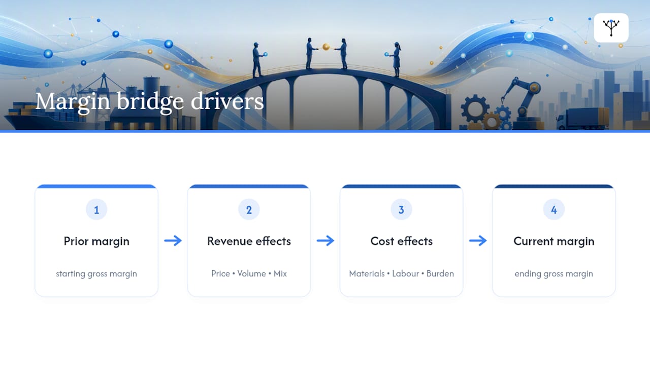
Six drivers explain almost every margin movement, and they split cleanly into two families. Price, volume and mix are revenue effects; materials, labour and burden are cost effects. Keeping these families separate is what lets you see offsetting movements, such as a price increase that looks great on the top line but gets quietly eaten by rising input costs.
Price is the trickiest of the six, because list price and net realised price are rarely the same thing. Net realised price is what actually lands after rebates, volume discounts and customer-specific terms are stripped out. A common hidden driver of margin decline is exactly this gap: reported list prices hold steady while discounting quietly widens, and nobody notices until the bridge forces the comparison at invoice level.
Volume measures what would have happened to margin if only unit quantities changed, holding price and mix constant. It's a counterfactual, not an observed figure. You build it by asking: if last period's price and product mix had applied to this period's volume, what would gross profit have been?
Mix captures the effect of selling a different blend of products, customers or channels, even if total volume barely moved. This is where the numbers can genuinely surprise you.
A single mix shift can swing blended margin more than a broad price change. Selling proportionally more of your highest-margin SKU, even with flat total units, can lift blended gross margin rate by a meaningful amount, according to worked examples from margin bridge modelling. That's why mix deserves its own line rather than being buried inside volume.
On the cost side, materials variance covers input price changes and usage efficiency, including the tariff exposure many manufacturers have felt acutely in recent years. Labour variance separates rate changes (wage inflation, overtime premiums) from efficiency changes (output per hour). Burden, the allocated overhead absorbed into unit cost, moves when volume changes shift fixed costs across more or fewer units, sometimes flattering margin in a way that has nothing to do with genuine operational improvement.
Step-by-step build: formulas, Excel layout and validation rules
Start with a clean baseline. You need prior-period and current-period figures at the most granular level your data supports, ideally SKU by customer by month: units sold, net revenue, and COGS. From those, calculate unit price (revenue ÷ units) and unit cost (COGS ÷ units) for both periods. Everything else in the bridge is built from these four numbers.
Revenue-side PVM formulas, using the standard approach from Coefficient's PVM guide:
- Price effect = (Current price − Prior price) × Current volume
- Volume effect = Prior price × (Current volume − Prior volume)
- Mix effect = (Current mix % − Prior mix %) × Total current revenue
That third formula treats mix as a share-of-total calculation, which works well when you're comparing product lines or customer segments within one total. Some analysts prefer a residual method instead, where mix is whatever's left after price and volume are removed from the total variance. Both are defensible; pick one and apply it consistently so period-on-period comparisons stay clean.
A pure revenue PVM tells you why sales moved, but it says nothing about profitability. A profit-focused PVM adapts the same three formulas by substituting unit margin (unit price minus unit cost) for unit price. This single adjustment is what turns a sales report into an actual margin bridge, because it shows whether a price increase was real profit or simply cover for rising costs.
Cost-side variance formulas mirror the revenue side. PVM logic applies equally well to COGS: materials rate variance, labour rate and efficiency variance, and burden absorption variance each follow the same current-volume-held-constant logic used on the revenue side. Combining a revenue PVM with a COGS PVM is what produces a genuine gross-margin bridge rather than two disconnected reports.
Suggested Excel layout:
- One row per SKU (or SKU × customer × month, depending on granularity), with prior-period and current-period columns side by side
- Calculated columns for unit price, unit volume, unit cost, and revenue/mix share in both periods
- A block of six output columns, one per driver, each populated with the formulas above
- A pivot table summarising the six driver columns by product line, region or whatever grouping your board wants to see
- A waterfall chart built from the pivot summary, starting at prior-period gross profit and ending at current-period gross profit
Numbered build steps:
- Pull transaction-level revenue, units and COGS for both periods into a single worksheet
- Calculate unit price and unit cost for every line in both periods
- Apply the price, volume and mix formulas to revenue
- Apply the equivalent formulas to COGS, splitting materials, labour and burden where your cost data allows
- Sum all six driver columns and compare the total to the actual period-on-period gross profit change
- Build the pivot and waterfall once the totals tie out, not before
Validation checks matter more than the formulas themselves. The sum of your six driver columns must equal the total gross profit change between the two periods, to the penny. If it doesn't, one of three things has usually gone wrong: a rounding error in the mix calculation, a scope change (an acquisition, a discontinued product line) that wasn't excluded or flagged separately, or an accounting policy shift (inventory valuation, cost allocation methodology) that moved the baseline without a corresponding driver to explain it. Add a residual line to your bridge and force yourself to explain it every time it's non-trivial.
Data preparation and common pitfalls for large datasets
Transaction-level data is messy, and PVM calculations are unusually sensitive to that mess. A handful of bad records can swing your mix effect by a wide margin without you noticing, because the formulas will happily calculate a result from garbage inputs.
Filter before you calculate, not after:
- Exclude SKUs with zero volume in either period; a brand-new product or a discontinued one will produce a nonsensical price variance if forced into the standard formula
- Strip out negative revenue lines and returns, or bucket them into their own explanatory column rather than blending them into the main analysis
- Flag one-off transactions (spot sales, clearance stock, error corrections) separately so they don't masquerade as a genuine price or mix trend
- Treat acquisitions, divestments and inventory policy changes as scope adjustments outside the six core drivers, with their own labelled bridge segment
FTI's guidance on this is unambiguous: filter zero-volume and negative-revenue SKUs out of the core calculation and categorise them separately rather than trying to force them through the standard PVM logic.
FX exposure and customer-specific pricing terms deserve particular care. If you sell internationally, calculate net realised price at invoice level, in the transaction currency where possible, before any FX translation blends currency movement in with genuine price action. Rebates and volume-tier discounts should already be netted out of your revenue figure; if they're not, your price driver will be measuring discounting policy rather than pricing power.
Pro Tip: Aggregate at the lowest level your patience allows, then roll up. Running PVM at SKU level and summarising into a pivot preserves far more signal than running the calculation on pre-aggregated category totals, where genuine mix shifts inside a category disappear entirely.
How to interpret drivers and translate them into management actions
A number on a bridge chart means nothing until someone owns it. The first question for every driver isn't "how big is it" but "will it persist or reverse." A one-off customer rebate that inflated last quarter's discounting will unwind naturally; a structural shift toward a lower-margin channel will not, unless someone actively intervenes.
Map each driver to an owner before the bridge reaches a board deck:
- Price erosion belongs with commercial or pricing leadership, who need to know whether it's deliberate discounting or unmanaged leakage
- Adverse mix belongs with sales leadership and category management, since channel and customer mix decisions usually sit with them
- Materials cost inflation belongs with procurement, who can renegotiate supplier terms or qualify alternative inputs
- Labour and burden variances belong with operations, where efficiency and absorption issues are typically solvable through scheduling or throughput changes
Prioritise by financial impact multiplied by ownerability. A driver worth £2 million that nobody can realistically influence this quarter (say, a currency movement) deserves a footnote, not a workstream. A driver worth £400,000 that procurement can address in six weeks deserves immediate attention.
Pro Tip: Watch for favourable mix masking cost inflation. It's one of the most common diagnostic traps in a margin bridge: total gross margin rate holds steady or even improves, but only because volume shifted toward higher-margin products while unit costs quietly rose across the board. Split the bridge by product line before declaring victory.
Price realisation erosion running alongside flat reported list prices is the other classic pattern worth a specific check: it almost always means discounting has drifted wider than sales leadership realises, and net realised price at invoice level will confirm it in minutes.
Reconcile and validate the bridge against the P&L and board reporting
Every column in your bridge should map to a specific line in the revenue and COGS sections of the P&L, and the reconciliation should be traceable enough that a finance director could follow it without asking you a single question.
Run these checks before the bridge leaves your desk:
- Confirm the six driver columns plus any residual sum exactly to the reported change in gross profit
- Check that FX translation effects are isolated, not blended into price or volume
- Confirm inventory timing (goods in transit, cut-off differences) hasn't created a phantom volume effect
- Flag any accounting policy change (cost allocation method, standard cost revisions) as a named adjustment, never as part of the six core drivers
Present the result as a waterfall chart, starting at prior-period gross profit, stepping through each driver, and landing on current-period gross profit. Add footnotes for anything non-obvious, particularly residuals and scope adjustments; a board member who spots an unexplained bar will lose confidence in the whole chart faster than one who reads a clear footnote explaining a one-off inventory revaluation.
Concise worked example you can reproduce in Excel
Take two SKUs. Product A sold 1,000 units last period at £50 revenue and £30 cost per unit (£20 margin); this period, 900 units at £52 revenue and £31 cost (£21 margin). Product B sold 500 units last period at £80 revenue and £40 cost (£40 margin); this period, 700 units at £78 revenue and £42 cost (£36 margin).
Applying the profit-focused PVM formulas: Product A's price effect is roughly +£1,800, but its volume effect is negative, around −£2,000. Product B's volume effect is strongly positive, but its price effect is negative because unit margin fell. The mix effect captures the shift toward B's larger revenue share. Sum all six driver values across both SKUs and they should tie exactly to the total gross profit change, using the same Excel layout described earlier: rows per SKU, calculated driver columns, and a pivot rolling up to the waterfall.
How to operationalise margin bridge outputs
A bridge built once a quarter tells you what happened. The harder problem is catching price erosion or mix drift while it's still cheap to fix. A connected platform can integrate finance, sales and operations data into one live model, so margin signals surface as alerts against thresholds you set, with an owner attached automatically rather than discovered three weeks later in a board pack. Excel remains the right tool for a one-off deep dive or a board narrative; a connected platform earns its place when you want the same discipline running every week without rebuilding the spreadsheet each time. Read more on connecting finance and operations.
Presenting a margin bridge to executives
The mistake I see most often is a bridge that overclaims causality: six neat bars implying six clean, independent causes, when reality is messier. Reconciliation and traceability matter more to your credibility than a polished chart. My advice: end every bridge presentation with exactly two ownerable actions for the next review, not six. Executives remember two commitments. They forget a wall of variance colour.
— Ronan
Turn bridge findings into owned corrective action
Building the bridge is the analytical half of the job. The harder half is making sure price erosion, adverse mix or a materials cost spike gets an owner and a deadline before it repeats next quarter, rather than resurfacing as the same unexplained line in your next board pack. The finance data behind your bridge can be connected to operations and sales workflows that caused the movement, so a flagged driver becomes an assigned task with a threshold alert attached, not a static chart nobody revisits.

That matters most for managing directors and operations leaders juggling margin pressure across multiple product lines or sites, where a quarterly Excel exercise catches problems long after they've compounded. If your team already runs a solid PVM process and wants the same rigour running continuously with automated alerts and clear ownership, take a look at Oak & Nine for operations leaders and see how the platform maps your existing margin drivers to the people accountable for fixing them.
Sources
For deeper formula detail and template structures behind this guide, see FTI's PVM white paper, Finelo's gross margin bridge breakdown, Marquis Data's CFO framework, and Coefficient's Excel-ready PVM guide. For related operational context, see Oak & Nine's notes on improving margin strategy and cost-to-serve analysis.
- A Quantifiable Approach To Price Volume Mix Analysis | FTI
- Gross margin bridge: separating price, mix, volume and costs | Finelo
- Why did my gross margin change? CFO framework | Marquis Data